Intro to R and the Tidyverse
What is R?
R is a programming language designed for statistical computing. It is not just a statistics package: it is a language.
What is RStudio?
RStudio is a free R integrated development environment (IDE). It is cleaner and simpler than the default R GUI (graphical user interface). It has many useful features, like syntax highlighting and tab for suggested code auto-completion.
Additionally, it has a 4-pane workspace:
Top left window: the R code editor
Bottom left: interactive console
Top right window: shows your workspace, including a list of objects currently in memory, history tab
Bottom right: shows plots, external packages available on your system, files in your working directory, and help files
Useful RStudio shortcuts:
tab: auto-complete function
Ctrl+↑ or cmd+↑ (auto-complete tool that works only in the interactive console)
Ctrl+enter or cmd+return (executes the selected lines of code)
Things to keep in mind
R is case sensitive, so be careful while typing.
#is used for commentsKeyboard Shortcuts: Ctrl+Shift+C (Windows) Cmd+Shift+C (MacOS).
R does not care about spaces between commands or arguments.
Names should start with a letter and should not contain spaces.
You can use
.in object names (e.g.,my.data).Use forward slash (
/) in path names, even on Windows.
Working directory
Your working directory is the folder on your computer in which you
are working. We can find this with the getwd() command.
# Current working directory
getwd()
[1] /User/fordfishman/
We can also set our working directory with setwd(PATH).
# an example of the path to your workshop materials
# USE YOUR OWN PATH
setwd("Documents/Workshops/Intro to R and the Tidyverse 20220928/")
To see the files in your working directory, you can use
list.files().
list.files()
[1] "IntroR_Tidyverse_code_along.R" "IntroR_Tidyverse_code.R" "penguins.csv"
Creating Objects
However, it would be more useful if we assigned values to objects. We
create an object by giving it a name followed by the assignment <-
operator. You can make <- with the following shortcuts: Alt+-
(Windows) or Option+- (Mac).
weight_kg <- 60
weight_lb <- 2.2 * weight_kg
weight_lb # Print the value of weight_lb
[1] 132
We can also reassign our variables to new values, but be careful, as there is no warning given for this.
You can also remove a variable from your environment with the rm()
command.
weight_kg <- 100 # Overwrites your object. Be careful! no warning is given

rm(weight_lb) # Deletes that object
Storing many numbers as a vector
We can use c() to combine or concatenate values together into a
vector.
Myvector1 <- c(1,3,4,5) # c for combine/concatenate
Myvector2 <- c(1:7)
Myvector3 <- seq (1,6, by=0.5)

Myvector1
Myvector2
Myvector3
[1] 1 3 4 5

[1] 1 2 3 4 5 6 7

[1] 1.0 1.5 2.0 2.5 3.0 3.5 4.0 4.5 5.0 5.5 6.0
You can also store characters and character vectors.
greeting <- "hello"
greeting

days <- c ("Sunday", "Monday", "Tuesday", "Wednesday", "Thursday", "Friday", "Saturday")
days
[1] "hello"

[1] "Sunday"    "Monday"    "Tuesday"   "Wednesday" "Thursday"  "Friday"    "Saturday"
To extract individual elements of a vector, we use an index in
square brackets. For instance, to get the third element of days, we
can use days[3]. Unlike other programming languages, R indexes from
1, not 0. Additionally, -1 will not get the last value: it excludes that
item.
days[3]
days[-1]
days[c(1,3)]
[1] "Tuesday"

[1] "Monday"    "Tuesday"   "Wednesday" "Thursday"  "Friday"    "Saturday"

[1] "Sunday"  "Tuesday"
Exercise 1
Extract Tuesday, Wednesday and Thursday from the days vector.
Solution
Note: these two solutions are equivalent.
days[c(3, 4, 5)]

days[3:5]
[1] "Tuesday"   "Wednesday" "Thursday"

[1] "Tuesday"   "Wednesday" "Thursday"
Replacing/adding new elements
We can also use indexing to replace or add new elements to a vector.
greeting[2] <- "How are you?"
greeting
Exercise 2
Replace the 3rd element in Myvector2 with a 10.
Solution
myvector2[3] <- 10
Data types
When we use c(), R assumes that everything in your vector is of the
same data type (all # or all characters).
Myvector4 <- c(1,2,"hello")
Myvector4
[1] "1" "2" "hello"
If we have different types of data we need to use the list()
function.
Mylist <- list(1,3, "hello", TRUE)

Mylist
[[1]]
[1] 1

[[2]]
[1] 3

[[3]]
[1] "hello"

[[4]]
[1] TRUE
Functions
A function is a piece of code to carry out a specified task. R has many built-in functions.
sum(1,3,5)
mean(Myvector1)
length(Myvector1)
max(Myvector1)
rep("hi", times=3)
[1] 9

[1] 3.25

[1] 4

[1] 5

[1] "hi" "hi" "hi"
If we want to learn more about a function we can ask for help with
help() or ?.
help(mean)
?rep
Packages
We can also bring in extra functions by downloading packages. Packages are collections of functions. There are thousands of add-on packages available at the CRAN (Comprehensive R Archive Network).
For instance, we have the tidyverse, an “opinionated collection of R packages designed for data science” (www.tidyverse.org). These packages are designed to make data wrangling, analysis, and graphing much simpler and more enjoyable.
Tidyverse packages share a philosophy of data organization: they all expect tidy data. Tidy data is set up so that each row is an observation and each column is a variable.
Using the tidyverse packages
To install a package we use the function
install.packages("package name"). We only need to install a package
once.
install.packages("tidyverse")
If we want to use the functions in a package, we need to load it in R
using the library() function.
library(tidyverse)
Importing data
Let’s explore penguins! In our file called penguins.csv, we have
data for three penguin species observed in the Palmer Archipelago,
Antarctica, collected by Dr. Kristen Gorman with Palmer Station LTER.
penguins <- read_csv("penguins.csv")
Exploring your data
We can use the View() function to look at our data frame.
View(penguins)
A very important function is str(), which lets you can view the
structure of data.
str(penguins)
spec_tbl_df [344 × 8] (S3: spec_tbl_df/tbl_df/tbl/data.frame)
$ species          : chr [1:344] "Adelie" "Adelie" "Adelie" "Adelie" ...
$ island           : chr [1:344] "Torgersen" "Torgersen" "Torgersen" "Torgersen" ...
$ bill_length_mm   : num [1:344] 39.1 39.5 40.3 NA 36.7 39.3 38.9 39.2 34.1 42 ...
$ bill_depth_mm    : num [1:344] 18.7 17.4 18 NA 19.3 20.6 17.8 19.6 18.1 20.2 ...
$ flipper_length_mm: num [1:344] 181 186 195 NA 193 190 181 195 193 190 ...
$ body_mass_g      : num [1:344] 3750 3800 3250 NA 3450 ...
$ sex              : chr [1:344] "male" "female" "female" NA ...
$ year             : num [1:344] 2007 2007 2007 2007 2007 ...
- attr(*, "spec")=
 .. cols(
 ..   species = col_character(),
 ..   island = col_character(),
 ..   bill_length_mm = col_double(),
 ..   bill_depth_mm = col_double(),
 ..   flipper_length_mm = col_double(),
 ..   body_mass_g = col_double(),
 ..   sex = col_character(),
 ..   year = col_double()
 .. )
- attr(*, "problems")=<externalptr>
We can get the same information using glimpse().
glimpse(penguins)
Rows: 344
Columns: 8
$ species           <chr> "Adelie", "Adelie", "Adelie", "Adelie", "Adelie", "Adelie", "Adelie", "Adelie", "Adelie", "Adelie…
$ island            <chr> "Torgersen", "Torgersen", "Torgersen", "Torgersen", "Torgersen", "Torgersen", "Torgersen", "Torge…
$ bill_length_mm    <dbl> 39.1, 39.5, 40.3, NA, 36.7, 39.3, 38.9, 39.2, 34.1, 42.0, 37.8, 37.8, 41.1, 38.6, 34.6, 36.6, 38.…
$ bill_depth_mm     <dbl> 18.7, 17.4, 18.0, NA, 19.3, 20.6, 17.8, 19.6, 18.1, 20.2, 17.1, 17.3, 17.6, 21.2, 21.1, 17.8, 19.…
$ flipper_length_mm <dbl> 181, 186, 195, NA, 193, 190, 181, 195, 193, 190, 186, 180, 182, 191, 198, 185, 195, 197, 184, 194…
$ body_mass_g       <dbl> 3750, 3800, 3250, NA, 3450, 3650, 3625, 4675, 3475, 4250, 3300, 3700, 3200, 3800, 4400, 3700, 345…
$ sex               <chr> "male", "female", "female", NA, "female", "male", "female", "male", NA, NA, NA, NA, "female", "ma…
$ year              <dbl> 2007, 2007, 2007, 2007, 2007, 2007, 2007, 2007, 2007, 2007, 2007, 2007, 2007, 2007, 2007, 2007, 2…
We can use some built-in functions in R to summarize the data, such as showing column names and the dimensions of the data frame.
class(penguins) # check to see that test is what we expect it to be
dim(penguins) # how many rows and columns?
names(penguins) # names of variables
[1] "spec_tbl_df" "tbl_df"      "tbl"         "data.frame"

[1] 344   8

[1] "species"           "island"            "bill_length_mm"    "bill_depth_mm"     "flipper_length_mm" "body_mass_g"
[7] "sex"               "year"
head() displays the first 6 rows of the data frame.
head(penguins) # first 6 rows
# A tibble: 6 × 8
 species island     bill_length_mm bill_depth_mm flipper_length_mm body_mass_g sex     year
  <chr>   <chr>              <dbl>         <dbl>             <dbl>       <dbl> <chr>  <dbl>
1 Adelie  Torgersen           39.1          18.7               181        3750 male    2007
2 Adelie  Torgersen           39.5          17.4               186        3800 female  2007
3 Adelie  Torgersen           40.3          18                 195        3250 female  2007
4 Adelie  Torgersen           NA            NA                  NA          NA NA      2007
5 Adelie  Torgersen           36.7          19.3               193        3450 female  2007
6 Adelie  Torgersen           39.3          20.6               190        3650 male    2007
tail() similarly shows the last 6 rows.
tail(penguins) # last 6 rows
# A tibble: 6 × 8
species   island bill_length_mm bill_depth_mm flipper_length_mm body_mass_g sex     year
<chr>     <chr>           <dbl>         <dbl>             <dbl>       <dbl> <chr>  <dbl>
1 Chinstrap Dream            45.7          17                 195        3650 female  2009
2 Chinstrap Dream            55.8          19.8               207        4000 male    2009
3 Chinstrap Dream            43.5          18.1               202        3400 female  2009
4 Chinstrap Dream            49.6          18.2               193        3775 male    2009
5 Chinstrap Dream            50.8          19                 210        4100 male    2009
6 Chinstrap Dream            50.2          18.7               198        3775 female  2009
We can use summary() to display some descriptive statistics, like
minimum and maximum values, means, and medians.
summary(penguins)
   species             island          bill_length_mm  bill_depth_mm   flipper_length_mm  body_mass_g       sex
Length:344         Length:344          Min.   :32.10   Min.   :13.10   Min.   :172.0     Min.   :2700   Length:344
Class :character   Class :character    1st Qu.:39.23   1st Qu.:15.60   1st Qu.:190.0     1st Qu.:3550   Class :character
Mode  :character   Mode  :character    Median :44.45   Median :17.30   Median :197.0     Median :4050   Mode  :character
                                       Mean   :43.92   Mean   :17.15   Mean   :200.9     Mean   :4202
                                       3rd Qu.:48.50   3rd Qu.:18.70   3rd Qu.:213.0     3rd Qu.:4750
                                       Max.   :59.60   Max.   :21.50   Max.   :231.0     Max.   :6300
                                       NA's   :2       NA's   :2       NA's   :2         NA's   :2
      year
Min.   :2007
1st Qu.:2007
Median :2008
Mean   :2008
3rd Qu.:2009
Max.   :2009
Note that the numerical variables are displayed different then the character variables. We can summarize the character variables better by converting them to factors.
penguins$species <- as.factor(penguins$species)
penguins$island <- as.factor(penguins$island)
penguins$sex <- as.factor(penguins$sex)
Here we access columns of a data frame using $, which is the easiest
way to do so.
penguins$species
penguins$island[1:10] # first 10
summary(penguins$body_mass_g)
 [1] Adelie    Adelie    Adelie    Adelie    Adelie    Adelie    Adelie    Adelie    Adelie    Adelie    Adelie    Adelie
[13] Adelie    Adelie    Adelie    Adelie    Adelie    Adelie    Adelie    Adelie    Adelie    Adelie    Adelie    Adelie
[25] Adelie    Adelie    Adelie    Adelie    Adelie    Adelie    Adelie    Adelie    Adelie    Adelie    Adelie    Adelie   ...
Levels: Adelie Chinstrap Gentoo

[1] Torgersen Torgersen Torgersen Torgersen Torgersen Torgersen Torgersen Torgersen Torgersen Torgersen
Levels: Biscoe Dream Torgersen

   Min. 1st Qu.  Median    Mean 3rd Qu.    Max.    NA's
   2700    3550    4050    4202    4750    6300       2
We can see the frequencies of a factor with table() or
summary().
table(penguins$species) # these give the same thing back
summary(penguins$species)
Adelie Chinstrap    Gentoo
   152        68       124
We can also sign numerical columns with a variety of functions.
mean(penguins$body_mass_g, na.rm=TRUE) # na.rm makes sure to ignore missing data
median(penguins$body_mass_g, na.rm=TRUE)
sd(penguins$body_mass_g, na.rm=TRUE)
[1] 4201.754

[1] 4050

[1] 801.9545
We can use the filter() tidyverse function to subset our dataframe.
Gentoo <- filter(penguins,species =="Gentoo")

Gentoo
# A tibble: 124 × 8
   species island bill_length_mm bill_depth_mm flipper_length_mm body_mass_g sex     year
   <fct>   <fct>           <dbl>         <dbl>             <dbl>       <dbl> <fct>  <dbl>
1 Gentoo  Biscoe           46.1          13.2               211        4500 female  2007
2 Gentoo  Biscoe           50            16.3               230        5700 male    2007
3 Gentoo  Biscoe           48.7          14.1               210        4450 female  2007
4 Gentoo  Biscoe           50            15.2               218        5700 male    2007
5 Gentoo  Biscoe           47.6          14.5               215        5400 male    2007
6 Gentoo  Biscoe           46.5          13.5               210        4550 female  2007
7 Gentoo  Biscoe           45.4          14.6               211        4800 female  2007
8 Gentoo  Biscoe           46.7          15.3               219        5200 male    2007
9 Gentoo  Biscoe           43.3          13.4               209        4400 female  2007
10 Gentoo  Biscoe           46.8          15.4               215        5150 male    2007
# … with 114 more rows
If we want to select specific columns, we can use the select()
function.
penguins_subsetted <- select(penguins, species, island, bill_length_mm, sex)
We can add new columns with mutate().
penguins_subsetted2 <- mutate(penguins_subsetted, mass_flipper_ratio = body_mass_g/flipper_length_mm)
We can use pipes to chain tidyverse commands together. Pipes in R
look like %>%. Read the pipe like the word “and then”.
female_penguins <- penguins %>%
   filter(sex == "female") %>%
   mutate(mass_flipper_ratio = body_mass_g/flipper_length_mm)
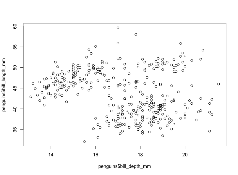
Simple graphs
To make a simple scatter plot in R, we can use the plot() function.
plot(penguins$bill_depth_mm, penguins$bill_length_mm)
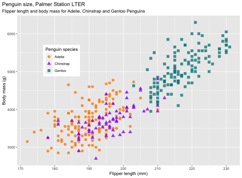
We can also use ggplot2 to get nicer graphs with many
customizations.
mass_flipper <- ggplot(data = penguins,
                       aes(x = flipper_length_mm,
                           y = body_mass_g)) +
   geom_point(aes(color = species,
                  shape = species),
                  size = 3,
                  alpha = 0.8) +
   scale_color_manual(values = c("darkorange","purple","cyan4")) +
   labs(title = "Penguin size, Palmer Station LTER",
         subtitle = "Flipper length and body mass for Adelie, Chinstrap and Gentoo Penguins",
         x = "Flipper length (mm)",
         y = "Body mass (g)",
         color = "Penguin species",
         shape = "Penguin species") +
   theme(legend.position = c(0.2, 0.7),
         plot.title.position = "plot",
         plot.caption = element_text(hjust = 0, face= "italic"),
         plot.caption.position = "plot")

mass_flipper