Pandas

Materials:

• Code-along Jupyter notebook

• Filled-in Jupyter notebook

While NumPy can be used to important data, it is optimized around numerical data. Many data sets include categorical variables. For these data sets, it is best to use a library called pandas, which focuses on creating and manipulating data frames.

Python

import pandas as pd

Read data

With pandas imported, we can read in .csv files with the pandas function read_csv().

In that function, we can specify the file we want to use with a URL or with the path to a local file as a string.

This saves the data in a structure called a DataFrame.

Python

df = pd.read_csv("https://raw.githubusercontent.com/DeisData/python/master/data/gapminder.csv") # read in data

Our data is now saved as a data frame in Python as the variable df. With the data now in the environment, we can take a look at the first few rows with df.head().

Python

df.head()

Output

	country	year	region	population	life_expectancy	age5_surviving	babies_per_woman	gdp_per_capita	gdp_per_day
0	Afghanistan	1800	Asia	3280000.0	28.21	53.142	7.0	603.0	1.650924
1	Afghanistan	1810	Asia	3280000.0	28.11	53.002	7.0	604.0	1.653662
2	Afghanistan	1820	Asia	3323519.0	28.01	52.862	7.0	604.0	1.653662
3	Afghanistan	1830	Asia	3448982.0	27.90	52.719	7.0	625.0	1.711157
4	Afghanistan	1840	Asia	3625022.0	27.80	52.576	7.0	647.0	1.771389

We can see that this data frame has several different columns, with information about countries and demography.

Summarize data frame

It is important to understand the data we are working with before we begin analysis. First, let’s look at the dimenions of the data frame using df.shape. It gives the number of rows by the number of columns.

Python

df.shape

Output

(14740, 9)

This shows that our data frame has 14740 rows by 9 columns.

We can also use df.columns to display the column names.

Python

df.columns

Output

Index(['country', 'year', 'region', 'population', 'life_expectancy',
       'age5_surviving', 'babies_per_woman', 'gdp_per_capita', 'gdp_per_day'],
      dtype='object')

Categorical variables

Next, let’s summarize the categorical, non-numerical variables. For instance, we can identify how many unique regions we have in the data set.

First, to select a column, we use the notation df['COLUMN_NAME'].

Python

df['region']

Output

0          Asia
1          Asia
2          Asia
3          Asia
4          Asia
         ...
14735    Africa
14736    Africa
14737    Africa
14738    Africa
14739    Africa
Name: region, Length: 14740, dtype: object

To identify unique entries in this column, we can use the .unique() function.

Python

df['region'].unique()

Output

array(['Asia', 'Europe', 'Africa', 'America'], dtype=object)

The countries column has many unique values, so instead of .unique(), we can use .nunique() to find the number of unique countries in the data set.

Python

df['country'].nunique()

Output

182

Numerical variables

Numerical columns can be summarized in several ways. Let’s find the mean first.

To make things simpler, we’ll just do calculations on the population, life_expectancy, and babies_per_woman columns. We can put those names in an arrangement called a list and then specify that list for the columns.

Python

num_cols = [ 'population', 'life_expectancy', 'babies_per_woman' ] # numerical columns

df[num_cols]

Output

	population	life_expectancy	babies_per_woman
0	3280000.0	28.21	7.00
1	3280000.0	28.11	7.00
2	3323519.0	28.01	7.00
3	3448982.0	27.90	7.00
4	3625022.0	27.80	7.00
...	...	...	...
14735	14255592.0	51.60	3.64
14736	14565482.0	54.20	3.56
14737	14898092.0	55.70	3.49
14738	15245855.0	57.00	3.41
14739	15602751.0	59.30	3.35

14740 rows × 3 columns

With this set of columns, we can run .mean() to find the mean of each column.

Python

df[num_cols].mean() # returns the mean of each column

Output

population          2.252933e+07
life_expectancy     5.683453e+01
babies_per_woman    4.643472e+00
dtype: float64

If we want a larger variety of summary statistics, we can use the .describe() method.

Python

df[num_cols].describe()

Output

	population	life_expectancy	babies_per_woman
count	1.474000e+04	14740.000000	14740.000000
mean	2.252933e+07	56.834526	4.643472
std	9.307143e+07	15.868464	1.994833
min	2.128000e+03	4.000000	1.130000
25%	8.990308e+05	44.230000	2.630000
50%	4.063978e+06	60.080000	5.060000
75%	1.218722e+07	70.380000	6.440000
max	1.376049e+09	83.300000	9.220000

We can also break down subgroupings of our data with the method .groupby().

Python

grouped_data = df.groupby('region')
grouped_data['population'].describe()

Output

	count	mean	std	min	25%	50%	75%	max
region
Africa	4293.0	9.181313e+06	1.655128e+07	12522.0	996331.00	3457113.0	9901052.00	1.822020e+08
America	2673.0	1.667833e+07	4.411806e+07	24000.0	331799.00	2843246.0	10061519.00	3.217736e+08
Asia	4212.0	4.604245e+07	1.658010e+08	2128.0	512028.25	4011309.5	19517390.25	1.376049e+09
Europe	3562.0	1.520351e+07	2.463153e+07	61428.0	2308682.00	5186801.5	10638884.75	1.484358e+08

Accessing rows and specific entries

You can also to access a specific row using df.loc[ROW, :]. The colon specifies to select all columns for that row number.

Python

df.loc[0, :] # the first row

Output

country             Afghanistan
year                       1800
region                     Asia
population            3280000.0
life_expectancy           28.21
age5_surviving           53.142
babies_per_woman            7.0
gdp_per_capita            603.0
gdp_per_day            1.650924
Name: 0, dtype: object

We can use .loc to find the value of specific entries, as well.

Python

df.loc[0, 'country'] # first row entry for column

Output

'Afghanistan'

Question 1: Summarizing data

Print out the summary statistics for columns age5_surviving, gdp_per_day, and gdp_per_capita.

Python

### your code below:

Solution

Python

df[['age5_surviving', 'gdp_per_day', 'gdp_per_capita']].describe()

Manipulate data

Subset by row

Sometimes, we want to create a subset of the main data frame based on certain conditions. We do this by using df.loc and specifying a condition for the rows.

Below, we take all of the rows where babies_per_woman is greater or equal to 4 with df['babies_per_woman'] >= 4 and assign this to a new data frame.

To check that this was done correctly, we can look at the minimum of the babies_per_woman column in the new data frame with .min().

Python

# take all rows where babies_per_woman is greater or equal to 4 and make a new data frame
df_4 = df.loc[df['babies_per_woman'] >= 4, :]
df_4['babies_per_woman'].min()

Output

4.0

We can use the following operators to make subsets: - Equals: == - Not equals: != - Greater than, less than: >, < - Greater than or equal to: >= - Less than or equal to: <=

We can also subset with categorical variables. Here, we take all rows where the country is Hungary.

Python

df_hungary = df.loc[df['country'] == 'Hungary', :]
pd.unique(df_hungary['country'])

Output

array(['Hungary'], dtype=object)

Math

If we multiply a data frame by a single number, each value in the column will be muliplied by that value.

Python

df['babies_per_woman'] * 1000

Output

0        7000.0
1        7000.0
2        7000.0
3        7000.0
4        7000.0
         ...
14735    3640.0
14736    3560.0
14737    3490.0
14738    3410.0
14739    3350.0
Name: babies_per_woman, Length: 14740, dtype: float64

We can also do math between columns, since they have the same length. Elements of the same row are added, substacted, multiplied, or divided.

Here, we subtract the life_expectancy column from the age5_surviving column and assign it to a new column called life_difference.

Python

df['life_difference'] = df['age5_surviving'] - df['life_expectancy']
print(df['life_difference'])

Output

0        24.932
1        24.892
2        24.852
3        24.819
4        24.776
         ...
14735    39.200
14736    37.130
14737    35.970
14738    34.900
14739    32.740
Name: life_difference, Length: 14740, dtype: float64

This new column is now reflected in the data frame.

Python

print(df.columns)

Output

Index(['country', 'year', 'region', 'population', 'life_expectancy',
       'age5_surviving', 'babies_per_woman', 'gdp_per_capita', 'gdp_per_day',
       'life_difference'],
      dtype='object')

Question 2: Working with data

Create a subset of data from Lithuania.

Within that subset, calculate the mean GDP per 1000 people across entries.

Hint: Multiply per capita GDP by 1000.

Python

### Your code here:

Solution

Python

df_lth = df.loc[df['country']=='Lithuania',:]
df_lth['gdp_per_1000'] = 1000 * df_lth['gdp_per_capita']
print(df_lth['gdp_per_1000'].mean())

Create your own data frame

To make your own data frame without a .csv, we use the function pd.DataFrame(). There are many ways to use this function to construct a data frame.

Here, we show how to convert a dictionary of lists into a data frame. Each list will be its own column, and you need to make sure the lists are all the same length. The keys of each list should be the column names.

Python

data_dict = {
   'a': [1, 3, 5],
   'b': ['apple', 'banana', 'apple'],
   'c': [-2., -3., -5.]
}

pd.DataFrame(data_dict)

Output

	a	b	c
0	1	apple	-2.0
1	3	banana	-3.0
2	5	apple	-5.0

You can also use lists of lists or 2D NumPy arrays to create data frames. Each list will be a row, instead of a column, and you will need to specify the column name as another argument in pd.DataFrame() called columns.

Python

data_list = [
   [1, 'apple', -2.],
   [3, 'banana', -3.],
   [5, 'apple', -5.]
]
pd.DataFrame(data_list, columns=['a', 'b', 'c'])

Output

	a	b	c
0	1	apple	-2.0
1	3	banana	-3.0
2	5	apple	-5.0

Note: we need to save this as a variable to use it in the future.

Sort data frame

To sort the rows in a data frame by the value of a column, we can use the .sort_values() method. The argument by requires a list with a column name.

Again, if you want to use the sorted version in the future, you need to save it as a new variable.

Python

my_df = pd.DataFrame(data_list, columns=['a', 'b', 'c'])

my_df.sort_values(by=['b'])

Output

	a	b	c
0	1	apple	-2.0
2	5	apple	-5.0
1	3	banana	-3.0

You can also sort descending by specifying the ascending=False argument.

Python

my_df.sort_values(by=['b'], ascending=False)

Output

	a	b	c
1	3	banana	-3.0
0	1	apple	-2.0
2	5	apple	-5.0

If desired, multiple column names can be specified, with priority given to those first in the list.

Python

my_df.sort_values(by=['b', 'a'], ascending=False)

Output

	a	b	c
1	3	banana	-3.0
2	5	apple	-5.0
0	1	apple	-2.0

Add rows

There are multiple ways to add a new row to a data frame. The most straightforward way is to use the pandas.concat() function with a new data frame with just one row.

We put the the two data frames into a list, and we set axis=0 to make sure it adds as a row. We will specify .reset_index(drop=True) to reset row numbers to account for the new row.

Python

new_row = pd.DataFrame({
   'a': [2],
   'b': ['banana'],
   'c': [-1.]
})

my_df2 = pd.concat([my_df, new_row], axis=0).reset_index(drop=True)

print(my_df2)

Output

   a       b    c
0  1   apple -2.0
1  3  banana -3.0
2  5   apple -5.0
3  2  banana -1.0

You can also use this approach to add multiple rows, as well, by having the new data frame consist of multiple rows.

Python

new_rows = pd.DataFrame({
   'a': [6, 5],
   'b': ['banana', 'orange'],
   'c': [-4., -9.]
})

my_df3 = pd.concat([my_df2, new_rows], axis=0).reset_index(drop=True)

print(my_df3)

Output

   a       b    c
0  1   apple -2.0
1  3  banana -3.0
2  5   apple -5.0
3  2  banana -1.0
4  6  banana -4.0
5  5  orange -9.0

Join data frames

A critical tool in data wrangling is combining data frames that share common values, columns, or identifiers.

Let’s important two new .csv files and join them.

Python

surveys_df = pd.read_csv("https://raw.githubusercontent.com/DeisData/python/master/data/surveys.csv", keep_default_na=False, na_values=[""])
species_df = pd.read_csv("https://raw.githubusercontent.com/DeisData/python/master/data/species.csv", keep_default_na=False, na_values=[""])

print(surveys_df.head())
print(species_df.head())

Output

   record_id  month  day  year  plot_id species_id sex  hindfoot_length  \
0          1      7   16  1977        2         NL   M             32.0
1          2      7   16  1977        3         NL   M             33.0
2          3      7   16  1977        2         DM   F             37.0
3          4      7   16  1977        7         DM   M             36.0
4          5      7   16  1977        3         DM   M             35.0

   weight
0     NaN
1     NaN
2     NaN
3     NaN
4     NaN

species_id             genus          species    taxa
0         AB        Amphispiza        bilineata    Bird
1         AH  Ammospermophilus          harrisi  Rodent
2         AS        Ammodramus       savannarum    Bird
3         BA           Baiomys          taylori  Rodent
4         CB   Campylorhynchus  brunneicapillus    Bird

The shared column between these data frames is species_id, so this is the column we will want to join around.

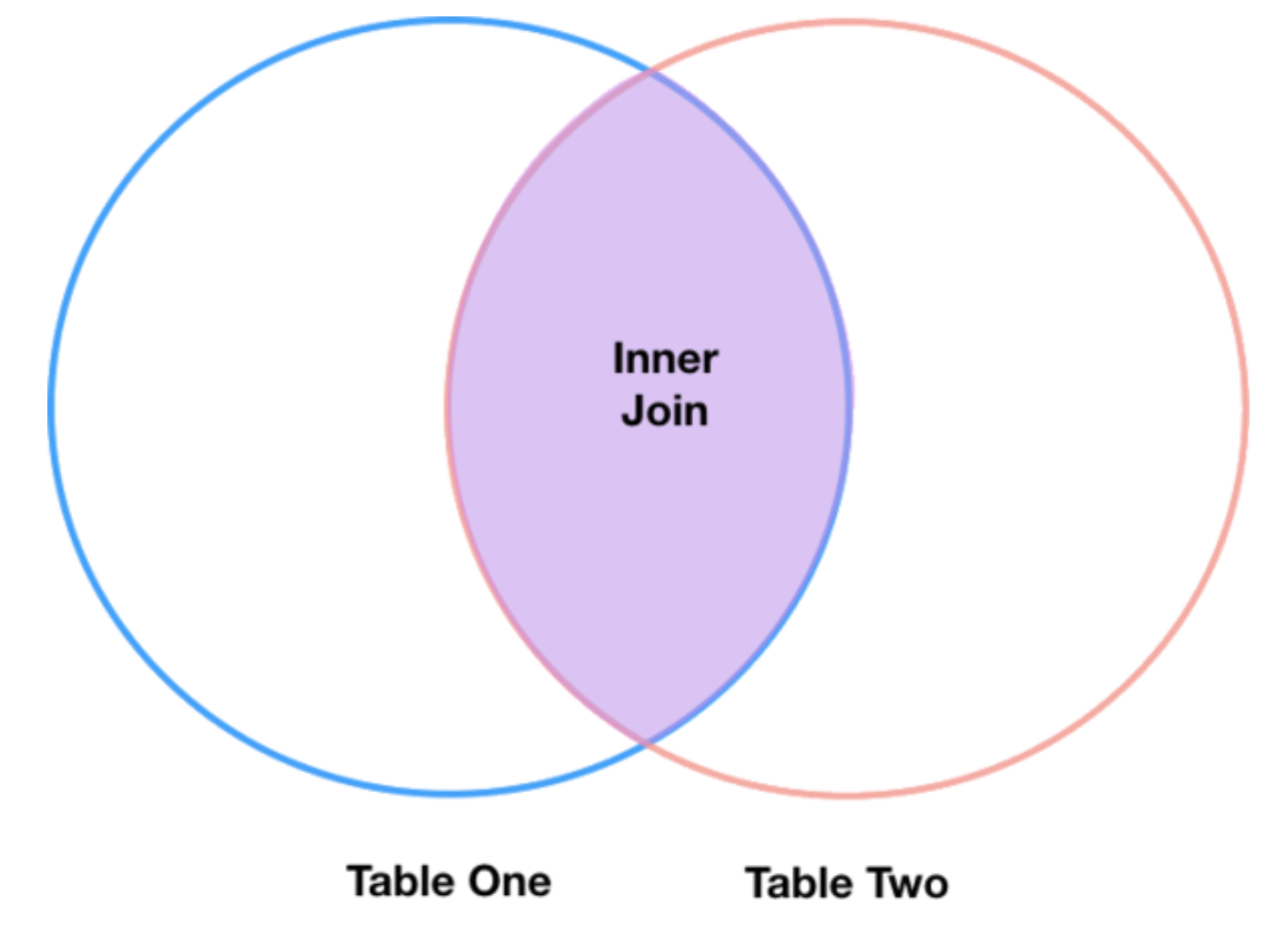
Inner Join

The pandas function for performing joins is called merge() and an Inner join is the default option.

Inner joins take all rows from both data frames that share values from an identifier column. In our case, this means that our joined data frame will only include rows with species identifiers present in species_df and surveys_df.

Python

merged_inner = pd.merge(left=surveys_df, right=species_df, left_on='species_id', right_on='species_id')

# In this case `species_id` is the only column name in  both dataframes, so if we skipped `left_on`
# And `right_on` arguments we would still get the same result

# What's the size of the output data?
print(merged_inner.shape)
merged_inner

Output

(34786, 12)

	record_id	month	day	year	plot_id	species_id	sex	hindfoot_length	weight	genus	species	taxa
0	1	7	16	1977	2	NL	M	32.0	NaN	Neotoma	albigula	Rodent
1	2	7	16	1977	3	NL	M	33.0	NaN	Neotoma	albigula	Rodent
2	22	7	17	1977	15	NL	F	31.0	NaN	Neotoma	albigula	Rodent
3	38	7	17	1977	17	NL	M	33.0	NaN	Neotoma	albigula	Rodent
4	72	8	19	1977	2	NL	M	31.0	NaN	Neotoma	albigula	Rodent
...	...	...	...	...	...	...	...	...	...	...	...	...
34781	28988	12	23	1998	6	CT	NaN	NaN	NaN	Cnemidophorus	tigris	Reptile
34782	35512	12	31	2002	11	US	NaN	NaN	NaN	Sparrow	sp.	Bird
34783	35513	12	31	2002	11	US	NaN	NaN	NaN	Sparrow	sp.	Bird
34784	35528	12	31	2002	13	US	NaN	NaN	NaN	Sparrow	sp.	Bird
34785	35544	12	31	2002	15	US	NaN	NaN	NaN	Sparrow	sp.	Bird

34786 rows × 12 columns

The result merged_inner data frame contains all of the columns from surveys_df (record_id, month, day, etc.) as well as all the columns from species_df (species_id, genus, species, and taxa).

Left join

What if we want to add information from species_df to surveys_dfwithout losing any of the information from surveys_df? In this case, we use a different type of join called a left join, where we keep all rows from the data frame we call left (in our case surveys_df) and only take rows from the right data frame (species_df) with species IDs in surveys_df.

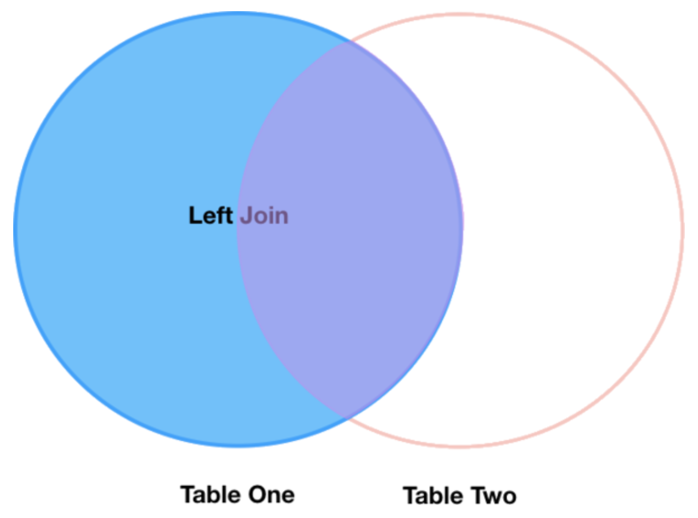
A left join is performed in pandas by calling the same merge() function used for inner join, but using the how='left' argument.

Python

merged_left = pd.merge(left=surveys_df, right=species_df, how='left', left_on='species_id', right_on='species_id')
merged_left

Output

	record_id	month	day	year	plot_id	species_id	sex	hindfoot_length	weight	genus	species	taxa
0	1	7	16	1977	2	NL	M	32.0	NaN	Neotoma	albigula	Rodent
1	2	7	16	1977	3	NL	M	33.0	NaN	Neotoma	albigula	Rodent
2	3	7	16	1977	2	DM	F	37.0	NaN	Dipodomys	merriami	Rodent
3	4	7	6	1977	7	DM	M	36.0	NaN	Dipodomys	merriami	Rodent
4	5	7	16	1977	3	DM	M	35.0	NaN	Dipodomys	merriami	Rodent
...	...	...	...	...	...	...	...	...	...	...	...	...
35544	35545	12	31	2002	15	AH	NaN	NaN	NaN	Ammospermophilus	harrisi	Rodent
35545	35546	12	31	2002	15	AH	NaN	NaN	NaN	Ammospermophilus	harrisi	Rodent
35546	35547	12	31	2002	10	RM	F	15.0	14.0	Reithrodontomys	megalotis	Rodent
35547	35548	12	31	2002	7	DO	M	36.0	51.0	Dipodomys	ordii	Rodent
35548	35549	12	31	2002	5	NaN	NaN	NaN	NaN	NaN	NaN	NaN

Export data frame as .csv

If you have made modifications to a data set in Python and want to export that to a new .csv, you can easily do that with the .to_csv() method that all pandas data frames have.

Python

%%script false --no-raise-error ## comment this line to run the cell

df_hungary.to_csv('gapminder_hungary.csv', index=False) # index = False makes sure row names are not saved as their own columns

Question 3: Putting it together

Create two data frames called A and B with at least 3 columns and 4 rows. Make one column in both A and B an identifier column, with at least one ID present in both data frames. Use a left join with A as the left data frame, and call the new data frame C. Display the data frame, and export it as a .csv file.

Python

### Your code here:

Solution

Python

A = pd.DataFrame({
   'ident': [0, 1, 2, 3],
   'size': [2.1, 5.2, 3.1, 1.5],
   'location': ['IL', 'MA', 'CA', 'NE']

})

B = pd.DataFrame({
   'ident': [5, 4, 0, 1, 3],
   'animal': ['monkey', 'giraffe', 'ape', 'lion', 'fish'],
   'sex': ['M', 'F', 'F', 'F', 'M']
})

C = pd.merge(left=A, right=B, how='left', left_on='ident', right_on='ident')
print(C)

C.to_csv('joined_data.csv', index=False)

Output

   ident  size location animal  sex
0      0   2.1       IL    ape    F
1      1   5.2       MA   lion    F
2      2   3.1       CA    NaN  NaN
3      3   1.5       NE   fish    M

Resources

• Pandas docs

• Pandas getting started

• Pandas cheatsheet

• PySpark for big data

This lesson is adapted from Software Carpentry.