Statistics with Python

Objectives

• Import data into a pandas data frame

• Import some standard and useful libraries for python

• Introduce some model fitting

Importing libraries and data

We will use several packages for our statistical analyses. In particular, we will use scipy.stats and statsmodels for running hypothesis testing and model fitting.

Python

   # Load standard libraries for data analysis
import numpy as np
import pandas as pd

import matplotlib
import matplotlib.pyplot as plt

# packages for statistics
import scipy.stats

import statsmodels
import statsmodels.api as sm
import statsmodels.formula.api as smf

%matplotlib inline

To find out more about a library and see the documentation, you can run ?LIBRARY_NAME.

Python

?scipy.stats

Describe and plot distributions

Let’s first import our GapMinder data set and summarize it.

Python

# Import data
gapminder = pd.read_csv('../data/gapminder.csv')
gapminder.info()

Output

<class 'pandas.core.frame.DataFrame'>
RangeIndex: 14740 entries, 0 to 14739
Data columns (total 9 columns):
#   Column            Non-Null Count  Dtype
---  ------            --------------  -----
0   country           14740 non-null  object
1   year              14740 non-null  int64
2   region            14740 non-null  object
3   population        14740 non-null  float64
4   life_expectancy   14740 non-null  float64
5   age5_surviving    14740 non-null  float64
6   babies_per_woman  14740 non-null  float64
7   gdp_per_capita    14740 non-null  float64
8   gdp_per_day       14740 non-null  float64
dtypes: float64(6), int64(1), object(2)
memory usage: 1.0+ MB

Python

gapminder

Output

	country	year	region	population	life_expectancy	age5_surviving	babies_per_woman	gdp_per_capita	gdp_per_day
0	Afghanistan	1800	Asia	3280000.0	28.21	53.142	7.0	603.0	1.650924
1	Afghanistan	1810	Asia	3280000.0	28.11	53.002	7.0	604.0	1.653662
2	Afghanistan	1820	Asia	3323519.0	28.01	52.862	7.0	604.0	1.653662
3	Afghanistan	1830	Asia	3448982.0	27.90	52.719	7.0	625.0	1.711157
4	Afghanistan	1840	Asia	3625022.0	27.80	52.576	7.0	647.0	1.771389
...	...	...	...	...	...	...	...	...	...
14735	Zimbabwe	2011	Africa	14255592.0	51.60	90.800	3.64	1626.0	4.451745
14736	Zimbabwe	2012	Africa	14565482.0	54.20	91.330	3.56	1750.0	4.791239
14737	Zimbabwe	2013	Africa	14898092.0	55.70	91.670	3.49	1773.0	4.854209
14738	Zimbabwe	2014	Africa	15245855.0	57.00	91.900	3.41	1773.0	4.854209
14739	Zimbabwe	2015	Africa	15602751.0	59.30	92.040	3.35	1801.0	4.930869

14740 rows × 9 columns

Descriptive statistics

We can use built in functions in pandas to summarize key aspects of our data.

Python

max_pop = gapminder.population.max()
ave_bpw = gapminder.babies_per_woman.mean()
var_bpw = gapminder.babies_per_woman.var()

print('Max population:', max_pop)
print('Mean babies per woman:', ave_bpw)
print('Variance in babies per woman:', var_bpw)

Output

Max population: 1376048943.0
Mean babies per woman: 4.643471506105837
Variance in babies per woman: 3.9793570162855287

We examine quartiles using the .quantile() method and specifying 0.25, 0.50 and 0.75.

Python

gapminder.life_expectancy.quantile([0.25,0.50,0.75])

Output

0.25    44.23
0.50    60.08
0.75    70.38
Name: life_expectancy, dtype: float64

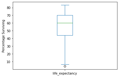
For very simple plots, we can plot directly from pandas, specifying the type of plot with the argument kind. Here we make a box plot and a histogram. We can then add labels with matplotlib.

Python

gapminder.life_expectancy.plot(kind='box')
plt.ylabel('Percentage Surviving')
plt.show()

Output

Python

gapminder.age5_surviving.mean()

Output

84.45266533242852

Python

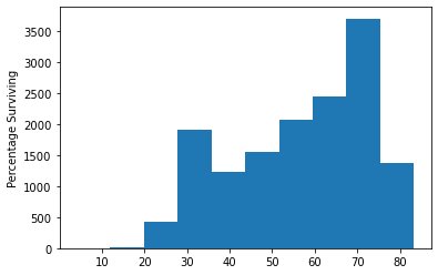
gapminder.life_expectancy.plot(kind='hist')
plt.ylabel('Percentage Surviving')
plt.show()

Output

Hypothesis Testing

Statistical methods are used to test hypotheses. One of the most foundational hypotheses we can ask is “Is the mean of this sample different from some value?” Typically, the value we are comparing the mean to has some sort of relavence.

While the actual mean of the sample might be different, we want to know if our data could have been generated if the true mean was a certain value. To do this, we use a 1-sample t-test.

To run a 1-sample t-test, we can use the ttest_1sample() function from the scipy.stats module.

Python

# 1 Sample t-test
# Is the mean of the data 84.4?
scipy.stats.ttest_1samp(gapminder['life_expectancy'], 57)

Output

Ttest_1sampResult(statistic=-1.2660253842508842, pvalue=0.20552400415951508)

If we want to compare the means in two samples, we need to run a 2-sample t-test, also called an independent samples t-test. We can use the function ttest_ind() for this.

Python

# 2 sample t-test
gdata_us = gapminder[gapminder.country == 'United States']
gdata_canada = gapminder[gapminder.country == 'Canada']

scipy.stats.ttest_ind(gdata_us.life_expectancy, gdata_canada.life_expectancy)

Output

Ttest_indResult(statistic=-0.741088317096773, pvalue=0.4597261729067277)

Fitting Models to Data

We have described the sample of a population with statistics. Now let’s understand what we can say about a population from a sample of data.

Python

# Get data subset
gdata = gapminder.query('year == 1985')
# grab population for point sizes
size = 1e-6 * gdata.population
# assign colors to regions
colors = gdata.region.map({'Africa': 'skyblue', 'Europe': 'gold', 'America': 'palegreen', 'Asia': 'coral'})

# create plotting function
def plotdata():
   gdata.plot.scatter('life_expectancy','babies_per_woman',
                     c=colors,s=size,linewidths=0.5,edgecolor='k',alpha=0.5)

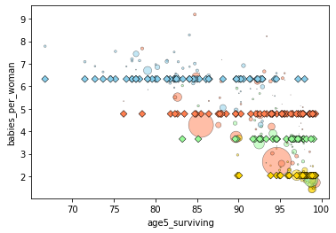
Using the custom function we just specified, let’s visualize the relationship between age5_surviving and babies_per_woman.

Python

plotdata()

Output

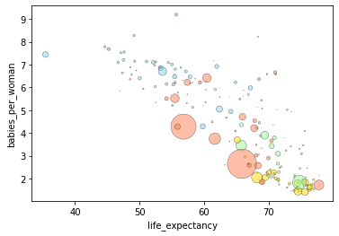
We can see there seems to be some sort of negative relationship between the two variables. There also might be a relationship between region and babies_per_woman, as well.

statmodels

statsmodels has many capabilities.

Here we will use Ordinary Least Squares (OLS). Least squares means models are fit by minimizing the squared difference between predictions and observations.

statsmodels lets us specify models using the “tilda” notation (also used in R) response variable ~ model terms.

For example: babes_per_woman ~ age5surviving.

Below we use the formula babies_per_woman ~ 1. This will essential just use the mean babies_per_woman value as the prediction for all data points.

Python

# Ordinary least squares model
model = smf.ols(formula='babies_per_woman ~ 1',data=gdata)
#    where babies per woman is the response variable and
#    1 represents a constant

# Next, we fit the model
grandmean = model.fit()

Let’s make a new function to visualize these results, using the old function we just made and adding in our predictions from our model on top.

Python

# Let's make a function to plot the data against the model prediction
def plotfit(fit):
   plotdata()
   plt.scatter(gdata.life_expectancy, fit.predict(gdata),
            c=colors,s=30,linewidths=0.5,edgecolor='k',marker='D')

plotfit(grandmean)

Output

Python

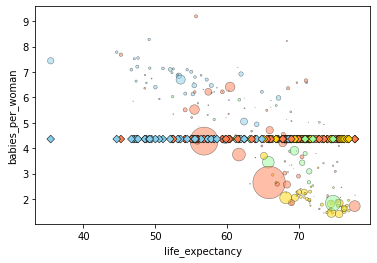
grandmean.params

Output

Intercept    4.360714
dtype: float64

Ever single data points get predicted to have the same value: 4.36. Thus, this is a very poor model.

Let’s try a slightly better model, using the region to preduct babies per woman. We use -1 in the formula to say we do not want to include a constant in the model.

Python

groupmeans = smf.ols(formula='babies_per_woman ~ -1 + region',data=gdata).fit()

plotfit(groupmeans)

Output

We can check the parameters of our fitted model to see the main effect of each region.

Python

groupmeans.params

Output

region[Africa]     6.321321
region[America]    3.658182
region[Asia]       4.775577
region[Europe]     2.035682
dtype: float64

An ANOVA can be used to test if these effects are significant.

Python

sm.stats.anova_lm(groupmeans)

Output

	df	sum_sq	mean_sq	F	PR(>F)
region	4.0	3927.702839	981.925710	655.512121	2.604302e-105
Residual	178.0	266.635461	1.497952	NaN	NaN

This is a much more informed model, but we can still do a lot better. Let’s take life_expectancy into account in a new model.

Python

surviving = smf.ols(formula='babies_per_woman ~ -1 + region + life_expectancy',data=gdata).fit()
plotfit(surviving)
print(surviving.params)

Output

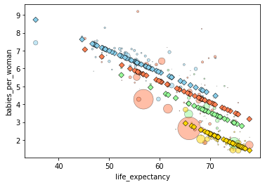
region[Africa]     12.953805
region[America]    11.885657
region[Asia]       12.452629
region[Europe]     10.703060
life_expectancy    -0.119281
dtype: float64

Now, we have a much better model.

statsmodels provides a summary for the fit with Goodness of Fit statistics, and also provides an anova table for the significance of the added variables.

Python

surviving.summary()

Output

OLS Regression Results

Dep. Variable:	babies_per_woman	R-squared	0.768
Model:	OLS	Adj. R-squared:	0.763
Method:	Least Squares	F-statistic:	146.9
Date:	Tue, 08 Nov 2022	Prob (F-statistic):	4.01e-55
Time:	10:18:04	Log-Likelihood:	-251.93
No. Observations:	182	AIC:	513.9
Df Residuals:	177	BIC:	529.9
Df Model:	4
Covariance Type:	nonrobust

	coef	std err	t	P>|t|	[0.025	0.975]
region[Africa]	12.9538	0.674	19.227	0.000	11.624	14.283
region[America]	11.8857	0.836	14.209	0.000	10.235	13.536
region[Asia]	12.4526	0.776	16.045	0.000	10.921	13.984
region[Europe]	10.7031	0.875	12.229	0.000	8.976	12.430
life_expectancy	-0.1193	0.012	-10.047	0.000	-0.143	-0.096

Omnibus:	19.859	Durbin-Watson:	1.967
Prob(Omnibus):	0.000	Jarque-Bera (JB):	37.777
Skew:	0.529	Prob(JB):	6.26e-09
Kurtosis:	4.965	Cond. No.	1.41e+03

Notes:[1] Standard Errors assume that the covariance matrix of the errors is correctly specified.[2] The condition number is large, 1.41e+03. This might indicate that there arestrong multicollinearity or other numerical problems.

We can also use the anova_lm() function with our model to estimate the importance of factors in our model.