Data Analysis

This section covers:

• Exploring and summarizing data

• Correlation and Chi-Squared tests

• T-test and ANOVA

• Checking assumptions

• Linear regression

Set up

To get started let’s install and/or load the libraries we will be using. If this is your first time using one of the packages “uncomment” and run the appropriate install.package(‘package’)

R

#install.packages('tidyverse')
library(tidyverse)
#install.packages('car')
library(car)
#install.packages('broom')
library(broom)
#install.packages ('rstatix')
library (rstatix)
#install.packages("sjPlot")
library(sjPlot)
#install.packages("lmtest")
library(lmtest)

We are going to analyze penguins! See https://allisonhorst.github.io/palmerpenguins/

Let’s get the data

R

install.packages("palmerpenguins")
library(palmerpenguins)

Exploring the data set

R

View(penguins)

We can check the structure

R

str(penguins)

Output

tibble [344 × 8] (S3: tbl_df/tbl/data.frame)
$ species          : Factor w/ 3 levels "Adelie","Chinstrap",..: 1 1 1 1 1 1 1 1 1 1 ...
$ island           : Factor w/ 3 levels "Biscoe","Dream",..: 3 3 3 3 3 3 3 3 3 3 ...
$ bill_length_mm   : num [1:344] 39.1 39.5 40.3 NA 36.7 39.3 38.9 39.2 34.1 42 ...
$ bill_depth_mm    : num [1:344] 18.7 17.4 18 NA 19.3 20.6 17.8 19.6 18.1 20.2 ...
$ flipper_length_mm: int [1:344] 181 186 195 NA 193 190 181 195 193 190 ...
$ body_mass_g      : int [1:344] 3750 3800 3250 NA 3450 3650 3625 4675 3475 4250 ...
$ sex              : Factor w/ 2 levels "female","male": 2 1 1 NA 1 2 1 2 NA NA ...
$ year             : int [1:344] 2007 2007 2007 2007 2007 2007 2007 2007 2007 2007

I want to see how many penguins I have

R

penguins %>%
 count(species)

Output

## # A tibble: 3 x 2
## species       n
## <fctr>      <int>
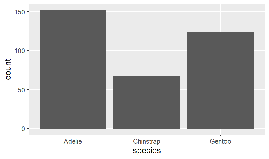
## Adelie             152
## Chinstrap       68
          ## Gentoo       124
          ## # 3 rows

Let’s create a bar graph

R

ggplot (penguins, aes(species))+
geom_bar()

Output

I want to see summary statistics for each species of penguin

R

penguins %>%
  group_by(species) %>%
    summarize(across(bill_length_mm:body_mass_g, mean, na.rm = TRUE))

Correlation

Is there a correlation between Flipper Length and Body Mass? Let’s create a scatterplot first

R

correlation_graph <- ggplot(penguins, aes(x = flipper_length_mm, y = body_mass_g)) +
geom_point() +
geom_smooth(method = lm)
correlation_graph

Output

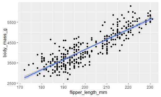
What’s the correlation coefficient?

R

cor.test(penguins$flipper_length_mm, penguins$body_mass_g)

Output

## # Pearson's product-moment correlation
## data:  penguins$flipper_length_mm and
## t = 32.722, df = 340, p-value <
## 2.2e-16
## alternative hypothesis: true correlation is
          ## not equal to 0
## 95 percent confidence interval:
## # 0.843041 0.894599
## sample estimates:
          ## # cor
## 0.8712018

Chi-Squared test

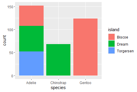
Now, I want to see if there is relationship between species and island. As both variables are categorical, we need to run a chi-squared test

Let’s visualize both varibles first

R

ggplot(penguins, aes(x = species, fill = island)) + geom_bar()

Output

We can also build contigency tables

R

penguins_table <- table (penguins$species, penguins$island)
penguins_table
prop.table(penguins_table)
prop.table(penguins_table, 1)*100
prop.table(penguins_table, 2)*100

Output

## #           Biscoe Dream Torgersen
## Adelie        44    56        52
## Chinstrap      0    68         0
## Gentoo       124     0         0
## #            Biscoe  Dream    Torgersen
          ## Adelie    0.1279070 0.1627907 0.1511628
## Chinstrap 0.0000000 0.1976744 0.0000000
## Gentoo    0.3604651 0.0000000 0.0000000
## #            Biscoe   Dream    Torgersen
          ## Adelie     28.94737  36.84211  34.21053
## Chinstrap   0.00000 100.00000   0.00000
## Gentoo    100.00000   0.00000   0.00000
## #            Biscoe  Dream    Torgersen
## Adelie     26.19048  45.16129 100.00000
## Chinstrap   0.00000  54.83871   0.00000
## Gentoo     73.80952   0.00000   0.00000

chi-squared test

R

chisq <- chisq.test(penguins$species, penguins$island)
chisq

Output

## #           Pearson's Chi-squared test
## data:  penguins$species and penguins$island
## X-squared = 299.55, df = 4, p-value < 2.2e-16

Independent Samples t-test

Is there a difference between males and females in their body mass?

Let’s visualize the data first

R

ggplot(na.omit(penguins))+
geom_boxplot(aes(x=sex, y=body_mass_g, fill=sex))+
theme_classic()+
ylab("Body mass")+
xlab('')+
theme(legend.position = 'none')

Output

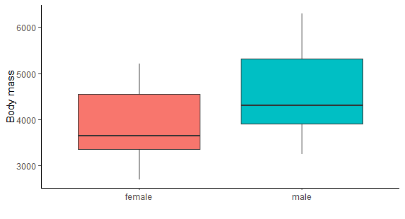
Are there any outliers? We can display these specific rows with the identify_outliers() function from the {rstatix} package

R

penguins %>%
group_by(sex)%>%
identify_outliers(body_mass_g)

Output

## 0 rows | 1-4 of 10 columns

We can check to see if the two samples have equal variance by performing a leveneTest, inside the functions we put a formula of the structure ‘continuous_variable ~ grouping’.

R

leveneTest(body_mass_g~sex, data=penguins)

Levene’s test has a null hypothesis that the variances are equal, based on the results of our test we reject the null hypothesis.

Output

## #  Levene's Test for Homogeneity of Variance (center = median)
##        Df F value  Pr(>F)
##group   1  6.0586 0.01435 *
##  331
## Signif. codes:
## 0 ‘***’ 0.001 ‘**’ 0.01 ‘*’ 0.05 ‘.’ 0.1 ‘ ’ 1

We will use the t.test() to compare the two means, the default for the function is to assume variances are not equal, and it performs a Welch Two Sample t-test. If we have equal variance we have to set the argument var.equal=TRUE which would run a Two-sample t-test.

R

t.test(penguins$body_mass_g ~ penguins$sex)

Output

## #  Welch Two Sample t-test
## data:  penguins$body_mass_g by penguins$sex
##t = -8.5545, df = 323.9, p-value =
##4.794e-16
## alternative hypothesis: true difference in means
##  between group female and group male is not equal to 0
## 95 percent confidence interval:
## -840.5783 -526.2453
## sample estimates:
## mean in group female   mean in group male
## 3862.273             4545.685

Effect Size. T-test conventional effect sizes: 0.2 (small effect), 0.5 (moderate effect) and 0.8 (large effect). For Welch t-test use ‘var.equal=FALSE’

R

penguins %>%
cohens_d(body_mass_g ~ sex, var.equal = TRUE)

Output

## # A tibble: 1 x 7
## .y.            group1  group2  effsize     n1   n2    magnitude
## <chr>           <chr>  <chr>   <dbl>       <int> <int>  <ord>
##1 body_mass_g   female  male    -0.9369085      165     168     large
          ## # 1 row

ANOVA: Comparing means from multiple groups

I would like to see if there are differences in the bill length between species.

We can start with a visualization

R

ggplot(penguins, aes(x = species, y = bill_length_mm)) +
geom_boxplot()

Output

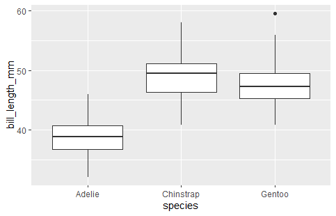
We can use the aov() function to run our anova. We will check our model assumptions after we fit the model. You want to assign the model fit to a variable name because we will use it to get the statistics and check assumptions.

R

anova<-aov(bill_length_mm~species, data=penguins)

summary(anova)

Output

## #            Df Sum Sq Mean Sq F value Pr(>F)
## species       2   7194    3597   410.6 <2e-16 ***
## Residuals   339   2970       9
## Signif. codes:
## 0 ‘***’ 0.001 ‘**’ 0.01 ‘*’ 0.05 ‘.’ 0.1 ‘ ’ 1
## 2 observations deleted due to missingness

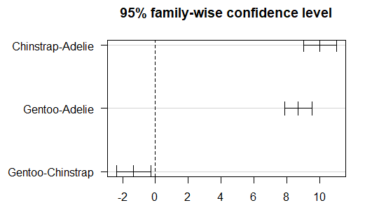
Post-Hoc analysis to see where the differences are

R

Tukey_test<- TukeyHSD(anova)
Tukey_test

Output

## #  Tukey multiple comparisons of means
## 95% family-wise confidence level
## Fit: aov(formula = bill_length_mm ~ species, data = penguins)
## $species
##                       diff       lwr        upr     p adj
## Chinstrap-Adelie 10.042433  9.024859 11.0600064 0.0000000
## Gentoo-Adelie     8.713487  7.867194  9.5597807 0.0000000
## Gentoo-Chinstrap -1.328945 -2.381868 -0.2760231 0.0088993

The tidyverse has a package called broom (we loaded this in earlier) and broom has a function called tidy() that we can use to create a cleaner table. We can also highlight significant differences with *

R

TukeyTidy<-TukeyHSD(anova)%>%
    tidy()%>%
    mutate(sig = case_when(adj.p.value < .05~ '*', TRUE ~''))
TukeyTidy

Output

## # A tibble: 3 x 8
## term contrast null.value estimate conf.low conf.high  adj.p.value  sig
## <chr> <chr>  <dbl>       <dbl>     <dbl>   <dbl>       <dbl>       <chr>
## species        Chinstrap-Adelie        0       10.042433       9.024859        11.0600064      0.000000000     *
## species        Gentoo-Adelie   0       8.713487        7.867194        9.5597807       0.000000000     *
## species        Gentoo-Chinstrap        0       -1.328945       -2.381868       -0.2760231      0.008899333     *
## 1-1 of 3 rows

We can also get a plot .. tab:: R

par(mar = c(3, 8, 3, 3))
plot(Tukey_test, las=1)

Output

Checking the homogeneity of variance assumption

R

leveneTest(bill_length_mm ~ species, data=penguins)

Output

## # Levene's Test for Homogeneity of Variance (center = median)
##         Df F value Pr(>F)
## group   2  2.2425 0.1078
## #        339

Checking the normality assumption

R

plot(anova,2)

Output

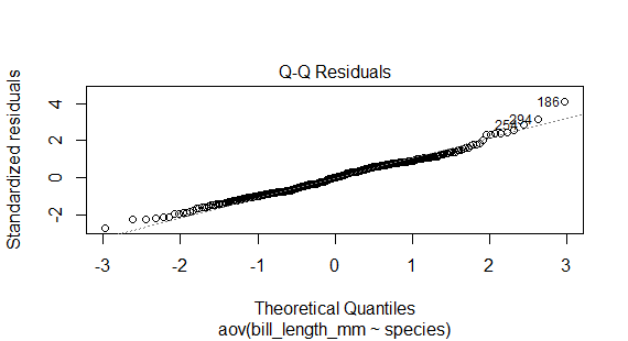
or we can use the Shapiro_Wilk test

R

anova_residuals <- residuals(object = anova )
shapiro.test(x=anova_residuals)

Output

## # Shapiro-Wilk normality test
## data:  anova_residuals
## W = 0.98903, p-value = 0.01131

The non-parametric alternative to one-way ANOVA is Kruskal-Wallis rank sum test, which can be used when ANNOVA assumptions are not met.

R

kruskal.test(bill_length_mm~species, data=penguins)

Output

## # Kruskal-Wallis rank sum test
## data:  bill_length_mm by species
## Kruskal-Wallis chi-squared = 244.14, df = 2, p-value <
## 2.2e-16

Linear Regression

A linear regression can be calculated the command lm. This function takes an R formula Y ~ X where Y is the dependent or outcome variable and X is the independent or predictor variable.

R

model1<-lm(body_mass_g ~ bill_length_mm, data=penguins)
summary(model1)

Output

## # Call:
## lm(formula = body_mass_g ~ bill_length_mm, data = penguins)

## # Residuals:
##     Min       1Q   Median       3Q      Max
## -1762.08  -446.98    32.59   462.31  1636.86
## Coefficients:
      ##         Estimate Std. Error t value Pr(>|t|)
## (Intercept)     362.307    283.345   1.279    0.202
## bill_length_mm   87.415      6.402  13.654   <2e-16 ***
## ---
## Signif. codes:  0 ‘***’ 0.001 ‘**’ 0.01 ‘*’ 0.05 ‘.’ 0.1 ‘ ’ 1

## Residual standard error: 645.4 on 340 degrees of freedom
##  (2 observations deleted due to missingness)
## Multiple R-squared:  0.3542,   Adjusted R-squared:  0.3523
## F-statistic: 186.4 on 1 and 340 DF,  p-value: < 2.2e-16

We can add more variables

R

model2 <- lm(body_mass_g ~ bill_depth_mm + flipper_length_mm, penguins)
summary(model2)

Output

## Call:
## lm(formula = body_mass_g ~ bill_depth_mm + flipper_length_mm,
## data = penguins)

## Residuals:
## Min       1Q   Median       3Q      Max
## -1029.78  -271.45   -23.58   245.15  1275.97

## Coefficients:
##                   Estimate Std. Error t value Pr(>|t|)
## (Intercept)       -6541.907    540.751 -12.098   <2e-16 ***
## bill_depth_mm        22.634     13.280   1.704   0.0892 .
## flipper_length_mm    51.541      1.865  27.635   <2e-16 ***
## ---
## Signif. codes:  0 ‘***’ 0.001 ‘**’ 0.01 ‘*’ 0.05 ‘.’ 0.1 ‘ ’ 1

## Residual standard error: 393.2 on 339 degrees of freedom
##   (2 observations deleted due to missingness)
## Multiple R-squared:  0.761,    Adjusted R-squared:  0.7596
## F-statistic: 539.8 on 2 and 339 DF,  p-value: < 2.2e-16

…and compare our models with the ‘tab_model’ function

R

tab_model(model1, model2, dv.labels = c("Model 1", "Model 2"))

Linear Regression assumptions

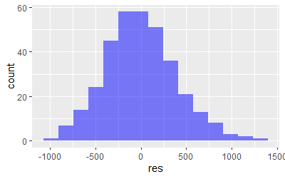
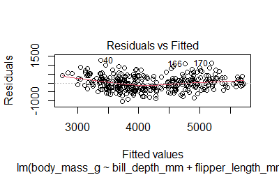
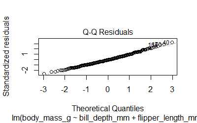
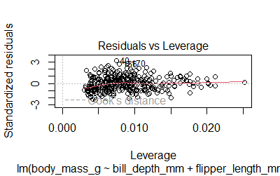
-Residuals are normally distributed. The plot()function will give us 4 diagnostic plots

R

res<-residuals(model2)
res <- as.data.frame(res)
ggplot(res,aes(res)) +
geom_histogram(fill='blue',alpha=0.5,bins=15)
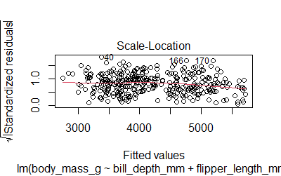
plot(model2)

Output

Output

Output

Output

Output

We can also run the Shapiro test

R

shapiro.test(model2$residuals)

Output

## # Shapiro-Wilk normality test
## data:  model2$residuals
## W = 0.99353, p-value = 0.1506

• Homoscedasticity. The variance of the residual in a regression model is constant.

We can check the Scale-Location plot or use the Breusch-Pagan test (null hypothesis: heteroskedasticity is not present)

R

bptest(model2)

Output

## # studentized Breusch-Pagan test
## data:  model2
##BP = 2.4223, df = 2, p-value = 0.2979

-Multicollinearity. This issue occurs when two or more independent variables are highly correlated. We can use vif() to calculate the variance inflation factor. A value larger than 2.5 may be a cause for concern.

R

vif(model2)

Output

## bill_depth_mm flipper_length_mm
##     1.51718           1.51718

Good resources to check out for more variations/details:

• R cookbook by Paul Teetor

• Learning Statistics with R by Danielle Navarro